
Introduction
The capital gains tax (CGT) discount was introduced in Australia in 1999 to simplify and incentivize investment in the share market. More recently, in the midst of a housing crisis, treasury has advised that the discount has a very small affect on home prices - of the order of 1-2% - and the current federal housing minister is on the record stating their policies aim for modest, stable residential real estate increases.
In this essay, I argue that these statements are mutually incompatible with analysis from modern portfolio theory. Specifically:
- while a CGT discount (combined with tax-deductable interest payments, a.k.a. negative gearing) incentivizes higher overall levels of investment, it also shifts the weighting of an optimal portfolio towards lower risk, lower volatility assets;
- this shift away from higher risk assets (like shares) can be larger than the increase in overall investment, resulting in less net investment in high risk assets; and
- these factors compound for low risk assets, resulting in a disproportionate effect.
Disclaimer
I am a mathematician and a computer scientist. While I’ve attempted to make things digestible where possible, I make no apology for including equations and graphs. If you understand quadratics, (somewhat) basic calculus and how to add random variables, nothing should be too magical. If not, hopefully the graphs are at least somewhat understandable.
The appendix contains materials for generating all plots and parameter values used.
Background
The Capital Gains Tax Discount
The capital gains tax discount was introduced after the 1999 Ralph Review suggested it would spur investment in risky assets. Specifically, it states:
The widespread privatization of major public sector enterprises has greatly increased the number of Australian households owning shares. A less harsh CGT regime which encourages taxpayers to invest in such assets will help entrench and build upon these changes. - Ralph Review
As an example, if somebody makes an investment that appreciates in value by \$100,000 and disposes of it after 1 year of holding, the capital gain is discounted by 50% before being added to the investor’s personal income. In this case, they would pay tax as if they had earned an additional \$50,000 (instead of the \$100,000).
Deductions and Negative Gearing
Costs associated with investments are generally considered tax deductible. This includes interest paid on geared (levered) investments. The practice of buying loss-making assets (like a lot residential real-estate) is hence known as negative gearing.
Tax Arbitrage
While both policies individually sound very reasonable, their combination allows for a tax arbitrage, where tax payers are incentivized to shift regular income into capital gains via leverage.
For example, if a tax payer on the top marginal rate (43%) makes and investment which costs \$110,000 to upkeep (e.g. interest payments), then sells the investment for a \$100,000 capital gain, the \$110,000 is deducted from their pre-tax income while only \$50,000 (50% of the \$100,000 capital gain) is added. As a result, they have a net \$60,000 tax deduction, resulting in a \$25,800 lower tax bill. Even after the \$10,000 loss (capital gain minus expenses) they end up \$15,800 ahead after tax.
This makes even poor investments - investments which cost more than they make - potentially profitable after tax. The best investment vehicles are those with strong capital appreciation and low interest rates, and it’s generally accepted that the best contender for that in the Australian investment landscape is residential real estate.
Banks, Treasury Modeling and Policy
Unsurprisingly, banks are only too happy to facilitate this arbitrage - for a fee. More than 60% of bank loans by value are tied to housing - roughly one third of which is for investment. This is largely consistent with ownership rates, with just over 30% of residential properties owned by investors.
Despite this, Treasury believes axing the CGT discount would have only a small effect on house prices - on the order of 1-2% - and the Housing Industry Association claims
The 1999 change to CGT did not have a tangible impact on… decisions by property investors.” - HIA
The current government’s official position that they would like house prices to continue growing “sustainably”.
Modern Portfolio Theory
Introduced in 1952, modern portfolio theory provides us a framework to compute optimal asset weightings and leverage for a rational risk averse investor. In this section we perform a quick review of a simple two-asset model before discussing the distortions resulting from the CGT discount.
Two Asset Case
Consider the simplified investment landscape featuring two different imperfectly correlated assets - one low risk, one high risk, with low and high expected returns respectively. I’ll be using expected return ($\mu$) and volatility ($\sigma$) figures ChatGPT suggested are typical of real estate and Australian shares, but the exact nature of the assets is largely irrelevant. While the real world is made up of significantly more than 2 types of assets, the results discussed here can be generalized thanks to the Two Fund Theorem, which essentially states that we can apply the theory below to the world of all possible asset classes by considering 2 mutual funds made up of different asset weightings.
Assets, Expected Returns, Volatility and Utility
We consider a rational risk-averse investor, meaning our investor will prefer a higher expected return over a lower expected return, and a lower volatility to a higher volatility. We can plot the assets as points on the $\sigma$-$\mu$ plane, understanding that our investor will prefer assets up and to the left (high returns $\mu$, low volatility $\sigma$).
Since our high risk asset has both higher expected returns and volatility, there’s no clear “better” option for a generic risk-averse investor - rather, it depends on how risk averse the investor is. If forced to choose just one, a highly risk averse investor will prefer the low risk investment, and an investor with low risk aversion will take the high risk asset. We parameterize an investor’s risk aversion level with some parameter $A \ge 0$ and combine the dual high return/low volatility preferences into a single preference for high utility given by
\[U = \mu - \frac{1}{2}A\sigma^2.\]Level curves of this function (plots of $\sigma$ vs $\mu$ for constant $U$) give us indifference curves, i.e. lines along which our investor will be equally happy.
\[\mu = U + \frac{1}{2}A\sigma^2.\]Just as before, our investor will always prefer to invest in assets up and left, but the level curves allow us to visualize the angle at which our investor’s utility increases greatest, normal to the level curve.
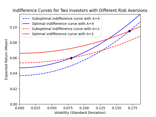
The above shows our investor with low risk aversion ($A = 2$, red lines) prefers the high risk, high expected return asset, since the utility of the solid red line (passing through the high risk asset, top right black dot) has a higher utility value ($y$-intercept) than the other indifference curve with the same $A$ passing through the low risk asset. The opposite is true of our highly risk averse investor ($A = 4$, blue lines).
Diversification
The “free lunch” of investing comes when we consider a portfolio made up of both our base assets. If we consider a combined asset made up of $(1 - \alpha)$ asset A and $\alpha$ asset B, the expected return is simple enough:
\[\mu(\alpha) = (1 - \alpha)\mu_a + \alpha \mu_b.\]The magic comes when we consider the volatility though:
\[\sigma^2(\alpha) = (1 - \alpha)^2 \sigma_a^2 + \alpha^2 \sigma_b + 2\alpha (1 - \alpha)\rho_{ab}\sigma_a \sigma_b.\]Unless you’ve done some statistics, that is not at all obvious. Without getting too side-tracked, the best intuitive analogy I can give is: think about the “volatility” of the result of rolling 2 dice and halving the result, and compare that to the volatility of rolling a single dice. In the first instance, your results will be much more closely grouped around 3.5 (i.e. the sum of two dice rolls more frequently give values like 6, 7 and 8 than 2 or 12, whereas the result of 1 dice roll is just as likely to give you a 1 or 6 as a 3 or 4).
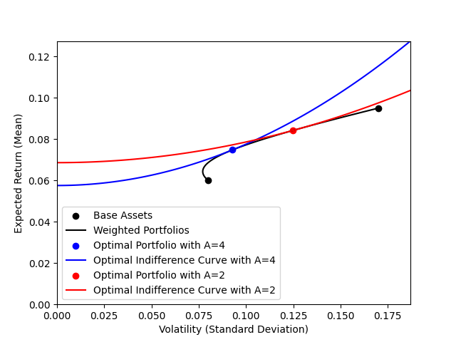
If we plot all possible portfolios made up of weighted combinations of base assets (black line) the “free lunch” can be seen by the movement up and left of our low risk asset. In other words, by adding a small amount of the high risk asset to our portfolio we both reduce the volatility AND increase the expected return. This is preferable for ALL rational investors regardless of their risk aversion parameter $A$. For specific risk aversion parameters, we can identify the optimal portfolio weighting by finding the specific utility $U$ for which the indifference curve is tangent to the portfolio line. Note for each risk aversion parameter, the optimal utility value ($y$-intercept) is higher than either individual asset ($y$-intercepts in the previous plot). As expected, our investor with lower risk aversion has an optimal portfolio weighting with more weight in the high risk asset than our investor with high risk aversion.
Adding a Risk Free Asset
Next, consider the case where we have access to a risk free investment. Traditionally large asset managers would use national treasury bills for this, but for our purposes we can think of them as an interest-bearing bank account or a loan. For simplicity we’ll assume we can borrow money at the same rate as we would earn interest, $r_f$.
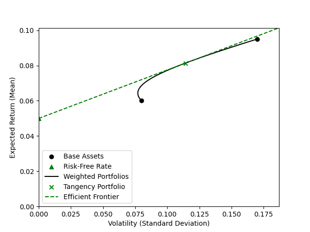
How does this affect our graphics above? Well, we can treat our risk free asset just like any other asset, with a mean $\mu$ and volatility $\sigma = 0$. Because of it’s risk free nature, the universe of assets made up of some weight of this and another base asset on the $(\sigma, \mu)$ plane is a straight line - and assuming there are no limits on how much we can borrow, we can extend this straight line forever. We denote this line the efficient frontier.
For any portfolio made up of a particular weighting of our low and high risk assets, we defines the Sharpe ratio $h$ as
\[h = \frac{\mu(\alpha) - r_f}{\sigma(\alpha)}.\]We define the tangency portfolio as the weighted portfolio with highest Sharpe factor, called such because it is tangent to the straight line from the risk free asset as shown below. As a result, it’s gradient is equal to the Sharpe factor.
Note the weight in this portfolio are independent of risk aversion. Just as previously though, we can use our risk aversion to determine a weighting between our risk free asset and our tangency portfolio. We call this weighting the leverage $\lambda$. A leverage value of $\lambda=1$ indicates no risk free asset. $\lambda < 1$ one indicates some money is invested in the risk-free asset, while $\lambda > 1$ indicates the risk-free asset is shorted - or in our bank account analogy, we have a loan. We compute the leverage by dividing the volatility of our target portfolio by the volatility of the tangent portfolio.
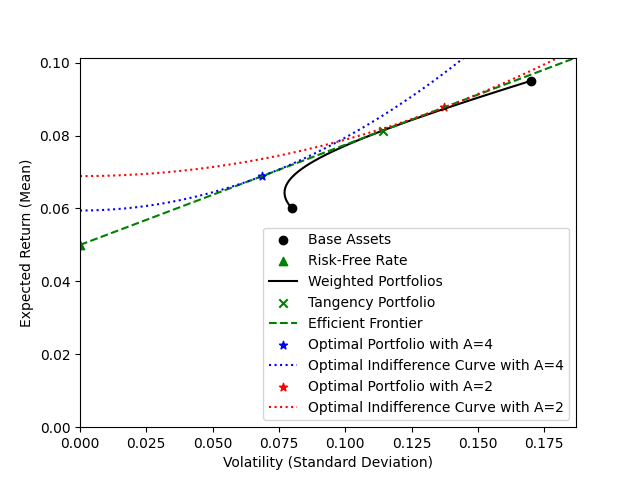
This shows that our highly risk-averse investor (blue) uses leverage $\lambda < 1$ since the blue star is to the left of the green cross, while our less risk-averse investor (red) uses leverage $\lambda > 1$ (the red star is to the right of the green cross). In other words, out risk-averse investor leaves some money in the bank uninvested, while our less risk-averse investor takes out a loan and invests that along with all their starting capital.
That’s a lot to digest, but the key take-aways are as follows:
- all investors should invest in the same weighted combination of low/high risk asset, determined by the combination with the largest gradient to the risk free asset / Sharpe ratio; and
- an investor’s risk aversion will dictate how much leverage to use.
Tax Distortions
The Australian tax system introduces two distortions:
- Negative gearing/tax payable on risk-free asset: if we consider after-tax income, this reduces both the income generated by capital in the risk free asset, and income paid on loans by a tax payer with marginal tax rate $t$ by $(1 - t)$.
- Capital gains tax, discounted by the discount factor $t_d = 50\%$, which reduces the expected return and volatility by a factor of $(1 - (1 - t_d)t)$ (assuming the investor has sufficient unrealized capital gains with which to offset any capital losses).
No tax vs Uniform Tax
First, let’s see how taxation in general affects investments. We’ll use the highest Australian tax bracket rate of $t = 43\%$ for an investor with risk aversion $A = 3$ and compare the difference between portfolios in a no-tax environment and a taxed environment. For the taxed environment case, we’ll consider everything in post-tax dollars, and assume interest paid is tax-deductable (and interest earned is taxed). We’ll also assume our investor has some unrealized gains which can be used to offset investment losses.
The effect of taxation on out $(\sigma, \mu)$ plane graphs is fairly boring: everything is scaled down by a factor of $1 - t$, including the Sharpe ratio (gradient of the efficient frontier). The tangency portfolio - i.e. the weighting between base assets - is the same in each case. Interestingly, the amount of leverage used differs, resulting in the taxed portfolio having the same volatility as the untaxed portfolio, but a lower expected return. That expected return is just the untaxed expected return reduced by the tax rate, so this is nothing unexpected.
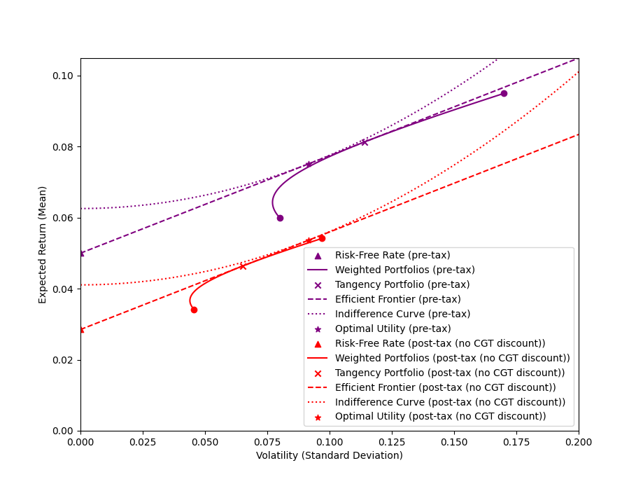
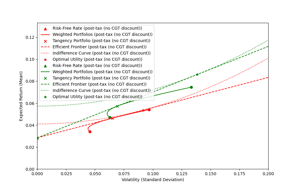
Uniform Tax vs CGT Discount
Things get interesting when we introduce the capital gains tax discount of $0 < t_d \le 1$ (set at $50%$ for the following diagrams). For simplicity, we assume our base asset returns are all capital gains, and the risk free asset is not (i.e. interest payments are treated as regular income when invested, and entirely tax deductible when paid). If we denote the tax rate on capital gain $t_\text{CGT} = (1 - t_d) t < t$ for some discount factor, our risk free rate is reduced by $(1 - t)$, while our base asset returns and volatility are reduced by $(1 - t_\text{CGT})$.
As shown above, introducing the CGT discount increases the Sharpe ratio/gradient of the efficient frontier and the tangency portfolio becomes more conservative (i.e. have more weight in the low risk asset). At the same time, the leverage used in the optimal portfolio increases.
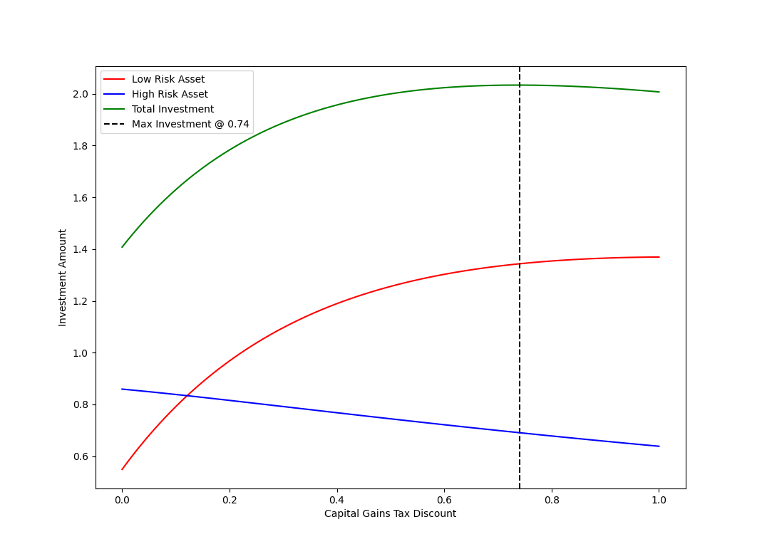
To see how the amount invested in each asset changes, we can plot the total amount in each base asset ($\lambda(1 - \alpha)$ and $\lambda \alpha$ for low and high risk assets respectively) for the optimal portfolio against the capital gains tax discount $t_d$. In this case, the $y$-intercepts represent the uniform (undiscounted) quantities.
Conclusions
We note the following:
- uniform tax does nothing to affect optimal asset allocation, though higher taxation results in higher levels of investment uniformly across assets;
- while overall investment levels increase with values of CGT discount up to $74\%$, it also moves investment from high risk assets to low risk assets;
- a capital gains tax discount of $50\%$ leads to roughly double the investment in the low risk asset;
- for high CGT discounts $t_d > 74\%$ the overall amount invested starts to decrease; and
- increasing the CGT discount from $50\%$ to $100\%$ would do little to increase overall investment, though a further shift from high risk assets to low risk assets would still occur.
If we assume investors are rational and accept the parameters used in this analysis, this means that the CGT discount has resulted in roughly double the amount invested than would otherwise be. Given that roughly a third of the real estate is currently owned by investors, this suggests roughly one sixth of real estate investment can be attributed to the CGT discount. I find it difficult to believe removing it would only result in a 1-2% drop in prices.
Appendix
Parameters Used
Except where otherwise specified, the following values were used in the above modeling.
| Parameter | Description | Value |
|---|---|---|
| $\mu_a$ | Expected return (mean) of low-risk asset | 6% |
| $\sigma_a$ | Volatility (standard deviation) of low-risk asset | 8% |
| $\mu_b$ | Expected return (mean) of high-risk asset | 9.5% |
| $\sigma_b$ | Volatility (standard deviation) of high-risk asset | 17% |
| $\rho_{ab}$ | Correlation between assets $a$ and $b$ | 0.2 |
| $t$ | Marginal tax rate | 43% |
| $t_d$ | CGT discount factor | 50% |
| $r_f$ | Pre-tax risk-free rate | 5% |
| $A$ | Risk aversion parameter | 3 |
Accompanying Resources
All plots and calculations are available in various forms below. The reader is encouraged to follow along and/or play around with parameters as desired.